Bittensor: A Peer-to-Peer Intelligence Market
Yuma Rao / Dr. Nick / 0xcacti
00/ Abstract
In this document, we present Dynamic TAO (DTAO): a market-driven mechanism designed to replace Bittensor's current emission allocation model. In particular, Dynamic TAO derives emission values from the market prices of subnet-specific tokens that trade against TAO on Constant Product AMMs. This fundamentally transforms the existing validator-weighting system. More specifically, by introducing AMM-based emission allocation, we extend the subnet valuation system beyond Bittensor's validator set to the rest of the Bittensor ecosystem, including miners and speculators. By replacing the current subnet valuation model with an open market, we make the subnet valuation process more efficient, increase coordination costs for malicious participants aiming to manipulate emissions, and eliminate the apathetic oligarchic voting system
- Section 1: Motivation
- Section 2: What is DTAO
- Section 3: Technical Overview
- Section 4: Mathematical Analysis
- Section 5: Appendix
This document will be presented in five sections:
Section 1: Motivation
Bittensor incentivizes the production and distribution of digital commodities by emitting newly minted TAO in each block to a set of subnets. This TAO is distributed to the subnets according to what is collectively referred to as the emission vector . Within each subnet, this emission is divided across three participant groups in the corresponding proportion:
- Validators (41%)
- Miners (41%)
- Subnet Owners (18%)
The details of the calculation are not important here, but roughly speaking, the emission vector is determined by the following calculation (where stands for the subnet):
The driving term in the above equation is the validator's favorability towards each subnet. Thus, these favorabilities essentially constitute a form of voting. Perhaps ideally, the weight vector resulting from this voting process would reward the subnets that are the most deserving, or those with the highest capital requirements. Problematically, the current system relies entirely on validators to manually assess and determine subnet value through their voting power. This creates a fundamental scaling problem: as the number of subnets grows, validators become increasingly unable to thoroughly evaluate each subnet's contribution to the network. The sheer volume of subnets requiring assessment often leads to validator apathy, where thorough evaluation becomes practically impossible.
This apathy can be further exacerbated by the lack of any meaningful consequences for validators who fail to maintain active and accurate weighting patterns. Indeed, the system provides no direct incentive for validators to regularly update their weight assignments or carefully consider their voting decisions. Even worse, the system incentivizes behavior that need not align with any ideal hypothetical weight distribution across subnets. As an example of a trivial way of manipulating the mechanism, validators may put more weight on subnets they actively validate upon in order boost their rewards (even if these are suboptimal subnets). Indeed, it would be merely altruistic for validators to provide weight to subnets on which they do not actively validate.
Another form of manipulation involves subnets owners offering revenue sharing agreements or other inducements to validators in exchange for larger weights on their subnet. Insidiously, this is a win-win scenario for the validators and subnet owners.
Fundamentally, the current incentive mechanism, with all of its flaws, can lead to less deserving subnets being rewarded in place of the more deserving subnets that would in fact accrue greater value to the Bittensor ecosystem. This is the motivation for introducing DTAO.
Section 2: What is DTAO
At it's core, Dynamic TAO (DTAO) is an upgrade to the Bittensor chain that replaces the previous emission logic with an intelligent, market-driven mechanism that can be used to determine token emissions. Operationally, we introduce subnet tokens (which we will informally refer to as Alpha1, Alpha2, Alpha3, etc.) through which miners, validators, and subnet owners will earn rewards. In so far as Bittensor enables the decentralized production and distribution of digital commodities, subnet tokens serve as the medium through which the network intelligently values these commodities. To facilitate this valuation, we also introduce subnet pools, which are Constant Product AMMs (described in details in section 3.1) through which users can stake TAO to receive subnet tokens and vice versa. The price discovery that occurs in these subnet pools functions as a view into how the Bittensor network values each subnet. Critically, this is exactly what we want, i.e. a scalable mechanism for valuing subnets that does not rely on a privileged, corruptible set of validators. Specifically, we will use the subnet token prices to guide the emission process.
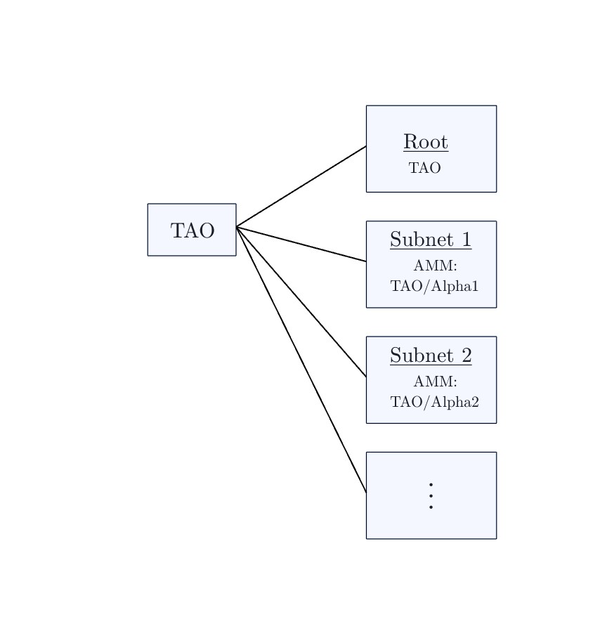
Figure 1: The Bittensor Subnets.
DTAO represents a fundamental shift towards true market democracy in the valuation of subnets. Where the previous system concentrated power in the hands of a few validators, DTAO opens participation to anyone willing to stake TAO in subnet pools. This broader participation not only makes the system more resistant to manipulation (try bribing a vast number of market participants for an extended period of time) but also ensures that subnet valuations reflect the collective wisdom of the market rather than the potentially biased views of a small group. Moreover, this market-driven approach scales naturally with network growth - as more subnets are added, the market simply expands to accommodate them, without degrading the quality of price discovery. Of course, this upgrade leads to a number of downstream changes, the core of which are discussed in detail in section (3.1) - (3.6), and the rest discussed in the appendix.
Section 3: Technical Overview
Section 3.0: A Look at the Components
In this section, we will look at some of the technical aspects of the DTAO system in a little more detail. There are many components to go over, so we will divide this section into five subsections, according to the following:
- (3.1) the AMM governing the subnet pools
- (3.2) the way in which new liquidity is injected
- (3.3) how TAO may be staked/unstaked from a subnet
- (3.4) the way that emissions are issued to users
- (3.5) the halving schedule
Additionally, there are several (less immediately relevant) technical sections reserved for the appendix.
Section 3.1: Subnet AMMs
Each subnet has its own liquidity pool allowing for swaps (and hence for price discovery) between the subnet-specific tokens and TAO. These pools will conduct swaps using the standard constant product AMM, and for this reason, we include a quick reminder of the relevant mechanics.
In a constant product AMM, we consider a liquidity pool containing two types of tokens, and we denote the total reserves of each by and . Swaps are conducted in a way to maintain the product of the token reserves. So, for a swap that changes the reserves by amounts , we must satisfy . This results in the viable states forming a hyperbola given by the equation , for some liquidity constant . Moreover, the spot price (i.e. the exchange rate ) is given by the ratio of the reserve amounts, These relationships, in turn allows us to write the reserves as and .
New liquidity can be added to a constant product pool in any number of ways. However, if we wish to maintain the current spot price, then the added amountsmust, themselves, be at the ratio of the current spot price. In other words, if we have and , then we will also have
For the remainder of this document, the subscript will be reserved for the subnet, and we will denote the subnet pool reserves by the following:
(`1`)
(`2`)
Indeed, we will sometimes informally refer to the subnet token simply as "Alpha." Moreover, we let denote the subnet token price denominated in TAO (i.e., the conversion from Alpha to TAO value). Then, from our discussion of the constant product AMM, we may write:
(`3`)
Section 3.2: Injections
At each block, an amount of Alpha and TAO tokens are to be added to the pool reserves. We call this an injection, and we denote these injection quantities by . These injection amounts are meant to reflect the relative performance of the subnets.There is no correct way to do this, but it is natural to imagine the subnet tokens as being speculative instruments, such that their prices correlate with subnet performances. We make the choice to define the subnet emissions along this line of reasoning.
To be precise, we fix a certain amount of total TAO to be emitted at each block, denoted , and we begin with the idea that this quantity should be divided among the subnets in proportion to their Alpha prices. In other words, the TAO injection for the subnet () would be given by the following:
(`4`)
When doing the injection, we don't want to artificially alter the subnet pool price. In other words, we should choose the corresponding Alpha injection () so that it maintains the ratio given in expression (`3). Specifically, this means that we must have the relationwhich then results in the following:
(`5`)
However, we will want to modify this formula based on the following observation:if the sum of pricesbecomes small, the Alpha injectioncan grow without bound.In order to prevent runaway inflation of the subnet tokens, we modify formula (`5) by putting a cap on the amount of Alpha emitted, which we will denote by (Note that this cap depends on the particular subnet depending on where the subnet is in its halving schedule—see Section 3.5.) Our injection formulas can then be summarized as follows:
(`6`)
(`7`)
We note two immediate consequences from these formulas:
(`8`)
(`9`)
Thus, we have firm upper bounds on the emission amounts.
The value of is initialized to be 1, to maintain the current emission schedule of 1 TAO per block. Similarly, for subnet tokens, we will takewhen each subnet is initialized, though all of these values are subject to halve according to the halving schedule (again, see section 3.5).
It should be noted that the minstatement in (`7) has the following effect: when the sum of all prices drops below a subnet-specific threshold (i.e., if), then less Alpha is emitted than would be needed to maintain pool price, and this drives the price of the pool up. This will be a critical feature in the early days of low liquidity when pool prices are more sensitive to movement.
Our injection formulas from (`6)-(`7) are presented in a way that is meant to be both readable and mathematically motivated. However, the way in which these quantities are computed in code is actually slightly different (while of course producing the same values). For the interested reader, we present the pseudo-code below. The variables tao_in and alpha_in represent the amount of tokens being injected into the subnet pool reserves, while the variable alpha_out represents the alpha to be emitted to the subnets, specifically as miner incentives and validator dividends. (One may note, the inject function not only injects liquidity into subnet pools, but it also delivers the alpha_out to the relevant parties.)
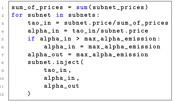
Figure 1: Injection pseudo-code
Lastly, it should be noted that when using the injection formulas in practice, we will actually use the exponentially weighted moving average (EMA) in place of the actual subnet pool price . This is done for several reasons:
- to discourage potential malicious attacks that can operate through price manipulation
- to smoothen out otherwise volatile price movements that may occur for low liquidity pools.
Section 3.3: Staking/Unstaking
If a user swaps some TAO on a subnet pool to obtain some subnet token (Alpha), then we say that the user stakes the TAO to the subnet. Similarly, if a user redeems their subnet token by swapping it for TAO, we say that the user unstakes TAO. Thus, the mechanics of staking and unstaking are relatively straightforward, as the rules for a constant product AMM are well established.
It should be noted, however, that different subnet tokens cannot be exchanged directly with each other. For example, if a user wishes to exchange some subnet token for other subnet token, they must first unstake some TAO from subnet (thereby relinquishing their)and then they must stake that TAO on subnet to obtain the desired amount
Lastly, it is worth noting that, unlike in typical AMMs, there will be no fees taken on the swaps, as there will be no liquidity providers to claim such fees. In other words, all liquidity of Alpha and TAO tokens is provided by the emission process.
Section 3.4: Subnet Emissions
Whereas validators, miners, and subnet owners were previously rewarded for their participation in the network through TAO, they will now be rewarded in Alpha. To accomplish this, we will have an additional quantity of Alpha, denotedthat is emitted at each block, and this quantity is to be divided up and distributed to users. For simplicity, we taketo be equal to the value(i.e. the maximum amount of Alpha injected into the pool per block, as previously defined).
(`10`)
Then the precise way in which we divide this quantity up can be described as follows:
- 18% go to subnet owners
- 41% go to miners
- 41% go to validators
- = the alpha outstanding is the total supply of Alpha held by users (not pool reserves).
- = the total TAO staked in the root subnet.
- = a freely chosen parameter that we call the tao weight, to be discussed momentarily.
- the fraction () is given to subnet validators
The Alpha emitted is divided up into three pieces, according to the ratio 41:41:18.
Next, we consider the the following quantities:
(`11`)
We use this ratio to split the validator dividends into two separate portions:
This process can be summarized in the following figure:
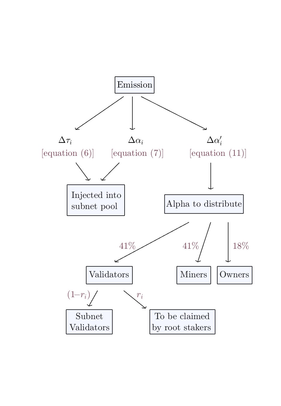
Figure 2: Flow chart of emission quantities
Now, one may wonder how we actually choose the value of this tao weight parameter. Generally speaking, the tao weight is meant to help smoothen the transition to the current DTAO design. In particular, there are a few guiding principles and motivations behind this parameter:
- We want to eventually transition from the current economic consensus to one fully governed by Alpha, but there are dangers in transitioning too quickly. In particular, the shifting supply and relatively low liquidity of the subnet tokens will drastically change in the first few months, and this can severely upset the existing consensus. However, with the tao weight parameter, we can slow this transition by diverting emissions to the root network initially, and we can keep the economic weight from shifting too fast. In the following figure, we plot the percent ownership of Alpha held by the root validators over time. This quantity naturally decreases over time, but the steepness of the curve varies depending on the specific chosen value of the tao weight:
- Though we do not discuss the consensus mechanism here, we note that the root proportion is also used to blend the stake weight (used in Yuma consensus) between TAO and Alpha. By tuning the value of the tao weight, we effectively have some control over the period where consensus transitions from being TAO dominated to being Alpha dominated. For example, if we instantly transition to a state of relying entirely on the Alpha stake for consensus, then as pools launch with low initial liquidity, it would be trivial for validators to try to quickly acquire Alpha and manipulate consensus on a given subnet. Thus, the tao weight allows us to prevent situations like this.
- The tao weight can prevent early Alpha holders from receiving absurdly high APYs. For example, note that if the tao weight is equal to zero (), then expression (12) tells us that the root proportion will also be zero (). Thus, from the flow chart above, it is clear that root stakers who do not own Alpha will receive no dividends at all in this case. One can easily work out that this results in a situation where the initial Alpha holders receive runaway dividends with shockingly high APYs (see figure 4).
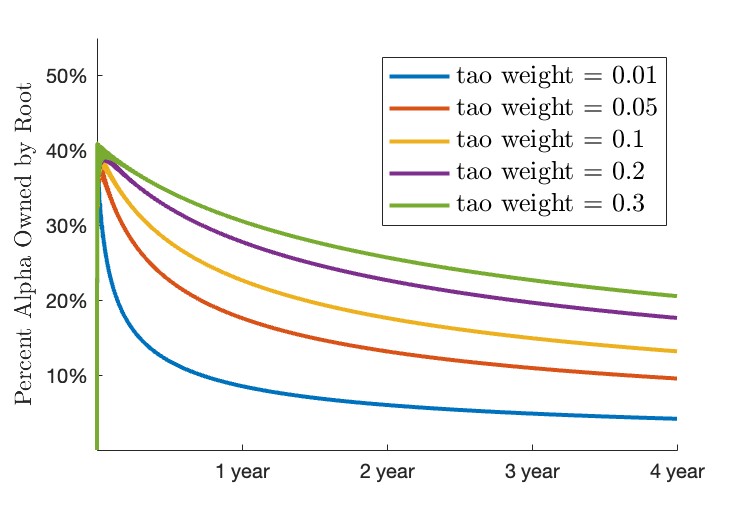
Figure 3: Root percentage ownership of Alpha over time
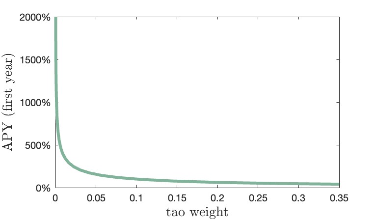
Figure 4: APY for early Alpha holders v.s tao weight
Section 3.5: Halving Schedule
The TAO halving schedule will remain unchanged from the previously established halving schedule. Specifically, the amount of TAO emitted per block is always equal to the quantity, and this quantity is subject to halve every time the accumulated TAO supply reaches certain supply thresholds. This causes the emission rate to halve roughly every four years (the details are provided in section 5.2).
New Alpha tokens will also follow the same halving schedule, with the emission amountbeing halved when reaching the same supply thresholds as TAO does (see appendix). Of course, the growth rate of Alpha supply can be up to double the value of, due to the fact that we inject some Alpha for the pool reserves (which is less than or equal to) as well as the emission amount (equal to ) for the rewards. Thus, while the growth rate of Alpha supply will be faster in time than that of the TAO supply, all halving events nevertheless occur at the same set of supply thresholds, and therefore every token supply approaches the same asymptotic value: 21,000,000. The following figure demonstrates this:
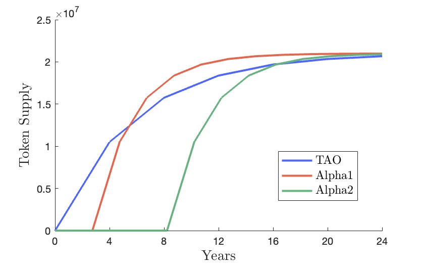
Figure 5: TAO and Alpha supply growth over time
Lastly, we note that as a consequence of the tapering rate of token supply growth, subnets that launch sooner in time will benefit from periods of faster liquidity growth in their subnet pools. Conversely, subnets that launch later in time must be content with slower liquidity growth.
Section 4: Analysis
In this section, we construct a simple mathematical toy model of the DTAO system, from which we may extract useful formulas for long term predictions. We will begin by establishing the governing rules for the model. We then make a few simplifying assumptions/approximations, and arrive at some useful formulas. Finally, we compare these formulas to some numerical simulations.
Section 4.1: Establishing a Dynamical System
To set the stage, we will assume that we have -many subnets (indexed by i) with constant product AMMs to swap between Alpha and TAO tokens. The token reserve quantities are denoted by, as functions of time:
(`12`)
(`13`)
As constant product pools, they obey the following:
(`14`)
(`15`)
where is the price of Alpha in terms of TAO, and is the liquidity scale factor for the pool. At regular intervals (blocks), the reserves update according to section 3.2:
(`16`)
(`17`)
The pool reserves are altered anytime a swap is executed, and these swaps then determine the pool price. However, for our mathematical model, we will suppose that the price trajectories are given (at least, probabilistically), and thus the pool reserves are determined implicitly. In particular, we note that while the liquidity factor is given by (16), it will also be determined simply by the cumulative amount of tokens injected. This is because swaps do not alter the liquidity constant (indeed, that is the whole point of the constant product), and so only the injection can determine . Thus, we define the cumulative token injections by the following:
(`18`)
(`19`)
With these defined, we can then restate L:
(`19`)
Finally, we define one more bit of notation for convenience. Specifically, we denote the sum of prices by
(`21`)
Then our deltas in (17)-(18) can be rewritten as
(`22`)
(`23`)
which will be slightly more convenient later on.
Section 4.2: Three Assumptions/Approximations
For our first simplifying assumption, we will assume that the prices each evolve according to Geometric Brownian Motion (GBM). Specifically, this means that for each subnet, we specify
- an initial price (0)
- a drift parameter
- a volatility parameter
and then the price at timewill be distributed with the following log-normal probability density:
(`24`)
Now, for a given set of parameters , our first goal will be to compute the expected values of , i.e., the cumulative injected tokens, up to some time :
(`25`)
(`26`)
To compute these, we accept the following approximation: we suppose the sums in (19)-(20) can be approximated as integrals. For example, with the expected cumulative Alpha in (27), we develop as follows:
(`27`)
This approximation should be reasonable since the sums happen over frequently occurring blocks, and are hence nearly continuous, while the rates and are constant and can simply be replaced with and . Next, we approximate the expected cumulative TAO:
(`28`)
Unfortunately, the appearance in the integrand of (28) and (29) makes them exceedingly difficult to calculate. In particular, depends on the entire set of prices , and so the expectation must be taken over the joint probability distribution of all of the -many price paths. Instead, we make our next approximation; we will replace with its expectation , denoted by .
(`29`)
The substitution is not completely unjustified; is a sum of approximately normal random variables, and by the generalized Central Limit Theorem, it will also be approximately normally distributed around its mean, with a relatively small variance over reasonably small time scales. Indeed, we will ultimately check it numerically.
Now, to compute the expectation of each price , we use the probability density given in (25).
(`30`)
With the change of variables , the integral in (31) can then be written as:
(`31`)
We can evaluate (32) by use of the standard formula
(`32`)
which can easily be derived by completing the square inside the exponential. Applying (33) to (32), we then find
(`33`)
Thus, expression (30) for then becomes
(`34`)
We note that, unlike the quantity , the quantity is not a random variable distributed with GBM, but is instead a deterministic function of . Thus, using our third approximation, we replace with in (28)-(29) and we find that it can now slip outside the expectation value:
(`35`)
(`36`)
We know that , and we knowfrom (34). Thus, (36)-(37) become:
(`37`)
(`38`)
Finally, we note that using
(`39`)
we can rewrite (38)-(39) in a more explicit way:
(`40`)
(`41`)
Our final approximation will be made in an effort to compute the expected market cap for each subnet pool. When denominated in TAO, the market cap of the subnet pool, denoted, is given by:
(`42`)
The price at time is of course given by . To calculate the total supply, we note that all the Alpha that can ever exist must come from the emissions. Thus, we simply need to add the cumulative emissions to any initial Alpha , and this will give us our total supply. However, for good measure we will also include the emissions that go to users as rewards. These rewards were not included in our toy model so far, but it is a trivial thing to include. We know from section 3.5 that an amount is emitted every block, and so the total amount up to time is (assuming is measured in blocks). Thus, our total expression for market cap will be given by:
(`43`)
Our interest will be in the expected market cap at time , and so we write the following:
(`44`)
Now, the expression would, in principle, be difficult to compute, as the expectation would be taken over the joint probability distribution of and . However, because of our approximation (30), the quantity is not actually a random variable. Thus, we may distribute the expectation over , obtaining:
(`45`)
Importantly, we see that expression (46) is written in terms of quantities that we have already worked out, namely (34) and (42). This will be our expression for the final market cap.
Summary So Far
Given prices with GBM parameters , and injection per unit time , the expected accumulated alpha and tao tokens , as well as the subnet market caps , at some time , are approximated by:
(`46`)
(`47`)
(`48`)
Section 4.3: Numerical Verification
To test our formulas, we run some numerical simulations. In particular, the purpose of the simulations in this section is simply to test the validity of our approximate expectation values given in (47)-(49). One should note, these will not be thorough agent-based simulations of the DTAO system in its full generality, but rather they are simulations of our idealized mathematical model articulated by the update rules (17)-(18), driven by simulated Geometric Brownian Motion price movements.
In order to completely visualize the results, we start with an unrealistically low number of subnets at
We use select the following drift and volatility parameters to generate a variety of price trajectories:
Over a period of years, and for all .We also note that this simulation does not include any halving events (indeed, the halving schedule was not factored in to our mathematical model from the previous section at all).
We now run 1,000 trials. For each trial, we generate four separate independent GBM price paths (one for each subnet) according to the values of and just given. First, we simply confirm the correct nature of our GBM by collecting the final prices for each subnet during each trial, and plot the distribution of final prices. For good measure, we also plot the log-normal distribution that we would mathematically expect for the probability density given in formula (25). The results are plotted in figure 6.
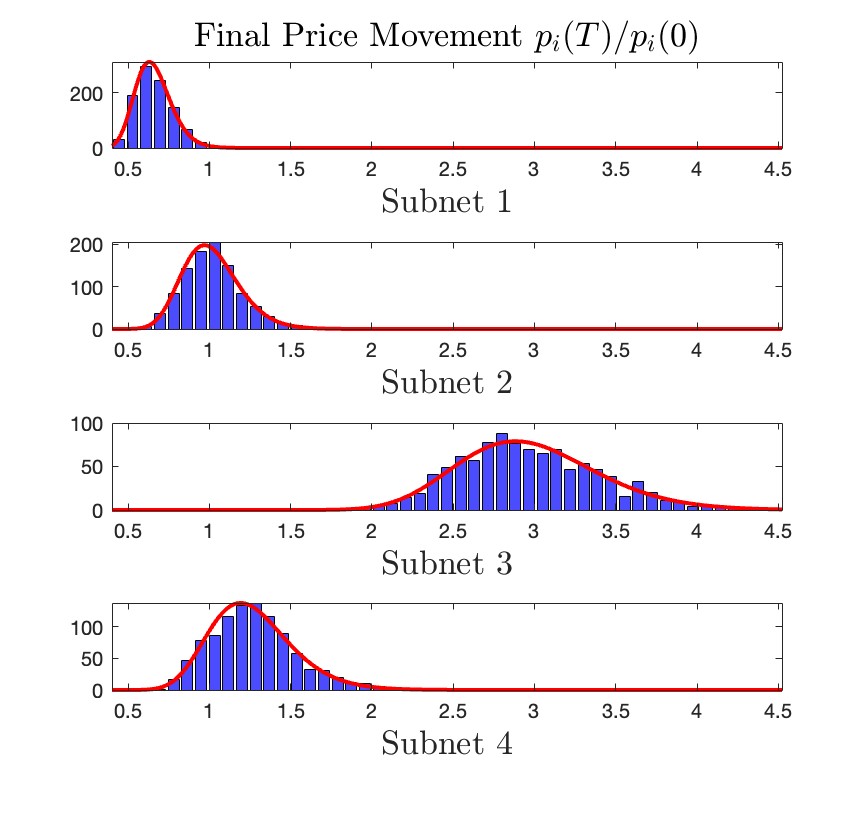
Figure 6: The distribution of final prices under GBM
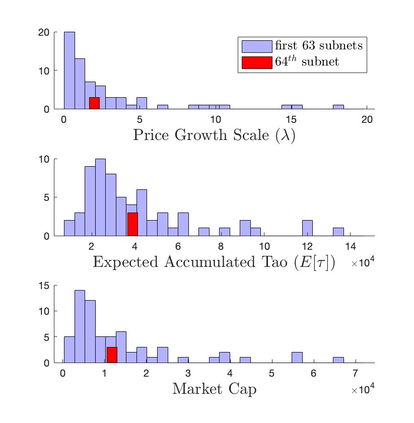
We next plot the distributions for our three quantities of interest; the cumulative injected Alpha and TAO tokens, and the final market cap, shown in figure 7 below. Indeed, we have markers to indicate the mean values from our raw simulation data, along with the values that our formulas (47)-(49) would predict. We make three observations:
- The data means agree excellently with our formulas
- The Alpha injections are identical for all subnets (this should be clear from the injection formula - it does not depend on , outside of ).
- The distributions of final prices, cumulative TAO, and market cap are all qualitatively similar.
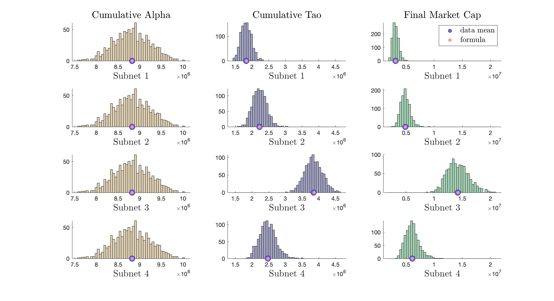
Figure 7: The distributions of final quantities
Section 4.4: Some Case Studies
Now that we feel confident in our expectation formulas , let us use them in specific case studies. We begin with a simple scenario wherein one subnet has a noticeable upwards drift in price, while the other subnet prices remain relatively stable. Specifically, we will use subnets, over a period year, with block emission of . We assign a normal spread of negligible drift parameters to the first 63 subnets, and we give the a noticeably higher drift. Moreover, we assign similarly mild random volatility parameters to all subnets. We can visualize these parameter assignments below:
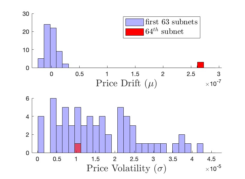
The drift parameter is hard to appreciate intuitively, but we convert it to the more relatable quantity (the price growth factor) by the equation . Using this, we plot the equivalent spread of values:
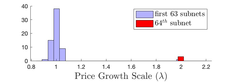
Thus, for example, our scenario corresponds with a subnet whose price doubles over the course of the year, while all other subnets move by about . Moreover, now that we have established the GBM setting, we use our formulas to compute expected values after one year. We plot the cumulative Alpha and TAO, and the final market cap:
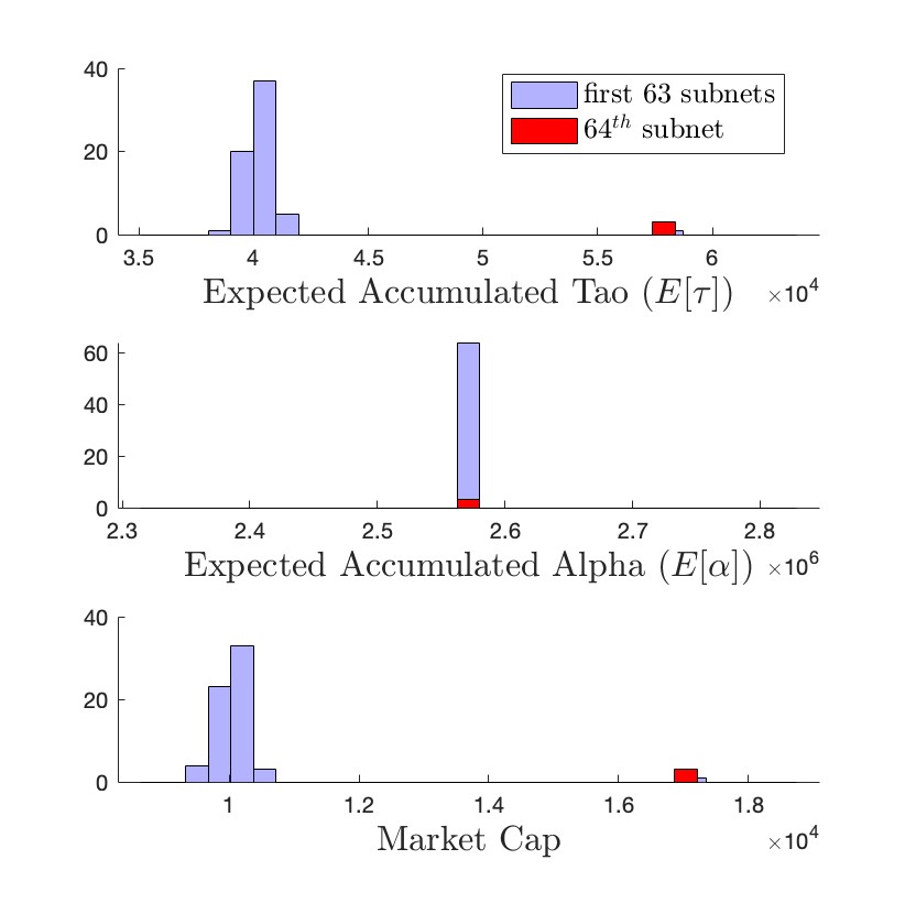
We can make a few observations from the previous figure. For our scenario with one subnet experiencing a doubling in price over the year, we can say the following:
- It will receive about more TAO tokens than the other subnets (note the values of for the general subnets, compared to for our special subnet; this is a increase).
- All subnets have the same expected cumulative Alpha tokens — again, not a surprise, as we previously noted.
- Our subnet can expect about 70% greater market cap at the end of the year
What if we give our subnet some competition? Let's take our previous scenario but suppose that there is a group of, say, ten other subnets who have similarly desirable drift parameters. We find the following:
Not surprisingly, our subnet now earns slightly less TAO and overall market cap than in the previous example.
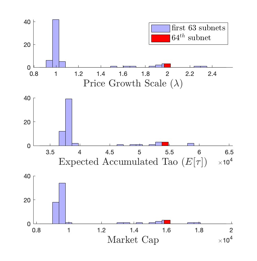
Finally, let us suppose that the subnets have a wide distribution of drift parameters, and that our subnet, while still experiencing a doubling of price, is situated somewhere in the middle of the pack. We find the following:
Armed with the formulas (47)-(49), the interested reader may investigate many more kinds of market trajectories and case studies beyond these simple scenarios.
Section 5: Appendix
Section 5.1: Tao Weight APY Differential
In this section, we explore an interesting heuristic to help guide us toward a good choice for the Tao weight . In particular, this heuristic will be based on comparing the APY earned by root stakers versus the subnet validators. As we saw in section 3.4, the amount of Alpha emission dedicated to the validators is given by . This is then split by the value of the root proportion into the following two pieces:
(`49`)
(`50`)
From our definition (12), we can write the following:
(`51`)
where we recall that
(`52`)
(`53`)
(`54`)
Now, for the Alpha outstanding term, we will make the following assumption; while Alpha may be coming in and out of the subnet pool, one could argue that if the subnet price remains relatively stable, then the Alpha outstanding should just be equal to the total cumulative Alpha emissions given out as dividends. Thus, starting at a value of , over a period of emissions, we employ the following simple model:
(`55`)
To get the APY, we would need to sum over appearing in (55) for the duration of a year. Rather than committing to a fixed time period, let us just consider generic returns. Moreover, to obtain these returns, we would divide the total rewards by the initial token held, i.e., either or. We do this next, while substituting (51) and (55) back into the reward expressions in (49) and (50). Altogether, we get the following expressions for the returns APY:
(`56`)
(`57`)
If we define
(`58`)
then (56)-(57) can be written more simply as
(`59`)
(`60`)
Now, to get the entire root returns, we would need to sum these rewards over all subnets, as the root stakers get dividends from each subnet:
(`61`)
Similarly, we could compute the average subnet returns by summing (57) over all subnets and dividing by the number of subnets (let's call it N):
(`62`)
We next suggest the following goal; let us choose the tao weight such that the root APY is less than or equal to the average subnet returns:
(`63`)
Explicitly, this becomes
(`65`)
This can be rearranged into the following:
(`66`)
We note that nearly every quantity in (65) is positive, except for the quantity . One way to guarantee that inequality (65) holds is to demand that . But this just simplifies to the following condition:
(`67`)
Thus, while this is surely a conservative choice, we can at least say the following:
If we take the tao weight to be the reciprocal of the number of subnets, then the root returns will be less than or equal to the average subnet returns
This could be a useful heuristic for choosing the tao weight, or at least gauge the appropriate order of magnitude.
Interestingly, we can use expressions (60) and (61) to get an approximate closed form expression for the return values. Specifically, if we replace the discrete sums with integrals (which is reasonable given how quickly the blocks happen), then we find the following:
(`67`)
(`68`)
Thus, we see that the subnet token holders have returns that grow linearly over time, whereas the passive root stakers have returns that only grow logarithmically .
Section 5.2: The Mechanics of Halving
In this section, we look at the math behind the halving schedule as computed in practice. We consider a scenario where we have an initial quantity (say, 1) that we add up N many times. After this point, we halve the quantity and add it up N many times again. This is done indefinitely:
This is meant to represent the accumulating token supply. For example, if we let , then we have the TAO halving schedule represented as the following:
(`69`)
Now, let us denote the current accumulated supply by . The eventual total token supply, which we denote by , will be given by using the well-known formula for summing a convergent geometric series:
and so we see that
(`70`)
Thus, for example, if , then we see that the total supply of TAO will approach .
Now, suppose we are currently at some point in this process, where the amounts being currently summed are , indicated below:
(`71`)
Let denote the accumulated supply up to the previous halving point, which we can sum as a finite geometric series:
(`72`)
In a similar way, we let denote the future accumulated supply at the point of the next future halving event.
(`73`)
We can solve equation (73) for the exponent k
(`74`)
We can do the same for equation (74) and solve for :
(`75`)
Now, because the current supply satisfies , and because the logarithm is a monotonically increasing function, then we can say the following:
(`76`)
In other words, we can compute k by the expression
(`77`)
Thus, at any point in time, we use the cumulative supply and the total target supply , and we can compute the amount of block emission according to (77).
Section 5.3: Root Reward Claiming (Accounting)
The root dividends (which are taken from the Alpha emissions) may be given to the root stakers in several ways. Initially, it will be done by auto-selling the dividends (in Alpha) into the subnet AMM and thus receiving TAO to then pass on to the root stakers (distributed on a pro-rate basis).
However, there may be a point when this is switched over to an alternative system where Alpha dividends are given directly to the root stakers as Alpha tokens. In this case, the Alpha dividends that are delivered to the root subnet accumulate and can be claimed at any point by users (again, on a pro-rata basis, depending on how much TAO they hold). In this section, we look at a particular kind of efficient accounting done for the root dividends. This is straightforward to compute and store in principle, but the efficient accounting method in use is somewhat opaque. To describe it, we define the following variables:
- = dividend injection of Alpha
- = TAO staked on root by a user
- = total TAO staked on root
- = a variable called 'rewards_per_tao'
- = a variable called 'debt'
- = Alpha that can be claimed by the user
Now, for an injection , a user is entitled to the quantity:
(`78`)
In other words, it's the fraction of the Alpha rewards that is equal by the user's fraction of TAO ownership. Next we define the following update formulas (where an apostrophe denotes an updated value):
(`79`)
(`80`)
(`81`)
(`82`)
We can confirm by induction that these formulas (77)-(80) achieve their desired goals. First, after an initial injection, equation (80) reduces to (76). Then, if we assume formula (80) holds for our inductive step, we consider another stake and/or injection. The amount that user should now be able to claim is . However, we can rearrange this:
(`83`)
which completes the inductive step.